Import Senzing Export to Excel & Formatting

Import Senzing Exported Data

The recommended method of importing exported CSV data from the Senzing App into Microsoft Excel is to use the From Text/CSV data tool.

• Open Excel, on the Data ribbon select the From Text/CSV tool
  
  
  
  
  
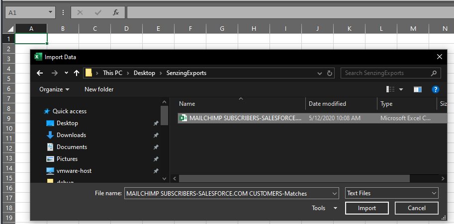
• In the Import Data file selection, choose the CSV file to import and click Import
  
  
  
  
  
• From the data transformation window click Load
  
  
  
  
  
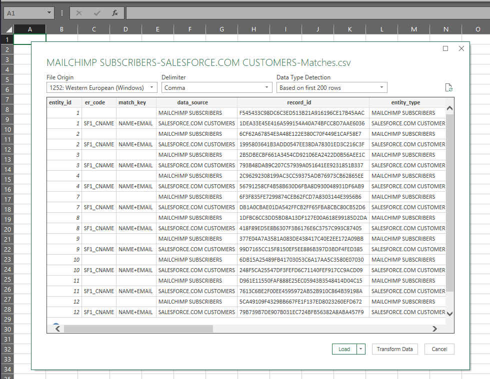
• The exported CSV is imported into Excel. Use the Table Design ribbon tools to format the table to your preferences.
  
  

Correcting Formatting of Newlines

Upon importing the CSV, some columns from the export can contain newline characters that don't appear to be effective in the Excel sheet. Consider the following and note the identifier_data column for Jeff Butcher contains both an EMAIL and NATIONAL_ID attribute concatenated together. 

If you examined the CSV file you would see there is a newline between these 2 attributes. To have Excel display these on separate lines within the row:

• Right click on the column header to reformat - in this instance identifier_data
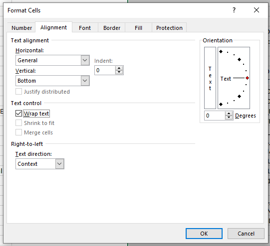
• In the Format Cells box navigate to the Alignment tab
• Under Text control select the tick box for Wrap text
• Click OK
  
  

Each distinct feature will now be on a separate row within the cell:

Formatting Rows Grouped by Entity ID

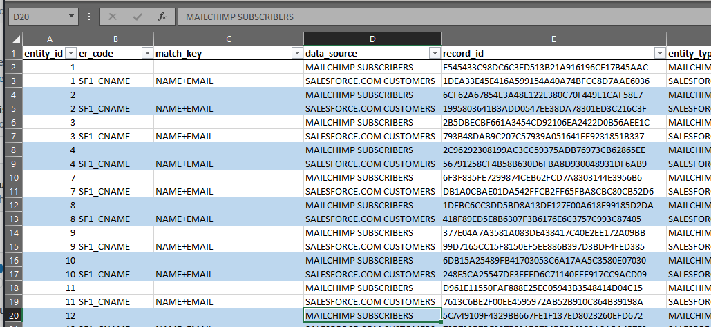
An additional tip is to use formatting to alternate the row fill color based on the ENTITY_ID column. This column indicates the similar records from within and across data sources ingested into Senzing that resolved together to form a single entity. Formatting the row color on this grouping value assists in visual interpretations of the results from the export. 

• Select row 2 by clicking the number 2 on the far left of the worksheet. Row 2 is selected because we do not wan't to consider the values in the header row.
  
  
  
  
  
• Hold the SHIFT + CTRL + DOWN ARROW keys to select all the remaining rows and columns in the sheet that contain data. 
  
  
• Navigate to the Home ribbon, select Conditional Formatting and New Rule... 
  
  
  
  
  
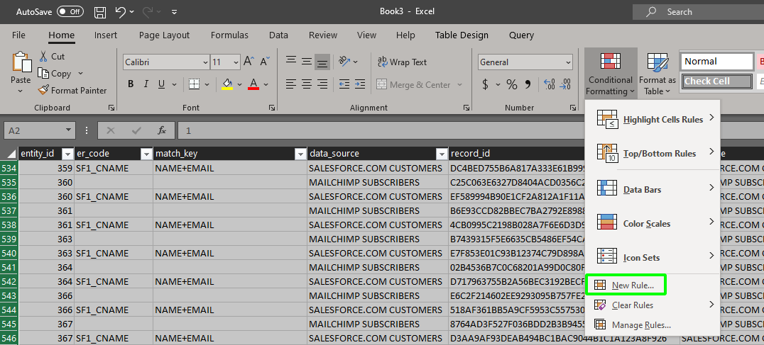
• In the New Formatting Rule box choose Use a formula to determine which cells to format, enter =ISODD(SUMPRODUCT(1/COUNTIF($A$1:$A2,$A$1:$A2))) in the Format values where this formula is true: entry and click Format... to choose your formatting preferences. 
  
  Click OK to apply.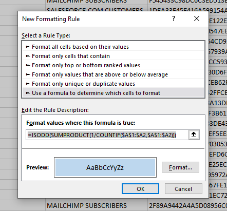 
  
  
  
  
  
  
• The sheet will now have the chosen formatting applied, grouped on the ENTITY_ID column.